RStudio project

Open the RStudio project that we created in the first session. I recommend to use this RStudio project for the entire course and within the RStudio project create separate R scripts for each session.

Create a new empty R script by going to the tab “File”, select “New File” and then “R script”
In the new R script, type # Session 12: MadingleyR, role of large carnivores and save the file in your folder “scripts” within your project folder, e.g. as “12_Mad_carnivores.R”

This practical illustrates how MadingleyR can be used to study top-down and bottom-up regulation of biomass across functional groups. As example, we re-implement parts of the large carnivore-removal case study described in (Hoeks et al. 2020). The workflow follows the example case study on herbivore-removal provided on https://github.com/MadingleyR/MadingleyR.

1 Large-carnivore removal scenario

Large terrestrial herbivores and carnivores are particularly vulnerable to extinction (Dirzo et al. 2014) while also being of vital importance for ecosystem structure and functioning (Svenning et al. 2016). Hoeks et al. (2020) used Madingley to investigate the importance of large carnivores for ecosystem structure and dynamics. They hypothesised that herbivores should increase in biomass when large predators are lost as the top-down regulation weakens and the bottom-up (resource) regulation strengthens.

To understand the effect of large carnivore removal on ecosystem structure and, thus, the importance of top-down control on the ecosystem, Hoeks et al. (2020) ran a simulation in which they remove all large (>21 kg) endothermic carnivores and compared this to a control, no-removal simulation. Here, we will not simulate global biomass differences, but just run the model for two 5x5° locations from Hoeks et al. (2020), Białowieża (Poland) and Serengeti (Kenya and Tanzania).

1.1 Setting up directory

We set up a directory to store all modelling results. Use your file explorer on your machine, navigate to the “models” folder within your project, and create a sub-folder for the current practical called “Mad_carnivores”. Next, return to your RStudio project and store the path in a variable. This has to be the absolute path to the models folder.

dirpath = paste0(getwd(),"/models/Mad_carnivores")

1.2 Initialise the model

First, we define the spatial windows for the two locations and initialise the model.

library(MadingleyR)

# Spatial window Bialowieza:
sptl_bialowieza = c(20, 25, 50, 54) 

# Spatial window Serengeti:
sptl_serengeti = c(32, 36, -4, 0)

# Initialise models for the two locations
mdat_B = madingley_init(spatial_window = sptl_bialowieza)

## Reading default input rasters from:  /Library/Frameworks/R.framework/Versions/4.1/Resources/library/MadingleyR/spatial_input_rasters.............
## Processing: realm_classification, land_mask, hanpp, available_water_capacity
## Processing: Ecto_max, Endo_C_max, Endo_H_max, Endo_O_max
## Processing: terrestrial_net_primary_productivity_1-12
## Processing: near-surface_temperature_1-12
## Processing: precipitation_1-12
## Processing: ground_frost_frequency_1-12
## Processing: diurnal_temperature_range_1-12
##

mdat_S = madingley_init(spatial_window = sptl_serengeti)

## Reading default input rasters from:  /Library/Frameworks/R.framework/Versions/4.1/Resources/library/MadingleyR/spatial_input_rasters.............
## Processing: realm_classification, land_mask, hanpp, available_water_capacity
## Processing: Ecto_max, Endo_C_max, Endo_H_max, Endo_O_max
## Processing: terrestrial_net_primary_productivity_1-12
## Processing: near-surface_temperature_1-12
## Processing: precipitation_1-12
## Processing: ground_frost_frequency_1-12
## Processing: diurnal_temperature_range_1-12
##

1.3 Run spin-up simulations and control scenario

We first let the model spin up for 50 years. Remember that this spinup phase should typically cover 100-1000 years; we shorten this for computational reasons in this demonstration. On my computer, this simulation runs through in 3-4 min (i.e. 0.20-0.25 sec per monthly timestep). Should it take much longer on your computer, you can reduce computational burden e.g. by reducing the maximum number of cohorts that are being simulated (in the madingley_run() function).

In the simulation, we define the maximum body masses of herbivores, carnivores and omnivores that are typically found at those locations (according to Table 2 of Hoeks et al. (2020)).

In contrast to Hoeks et al. (2020), we only run a single replicate per scenario.

# Define maximum body size of endotherms in the cohort definitions:
c_defs_B =c_defs_S = madingley_inputs('cohort definition')

c_defs_B$PROPERTY_Maximum.mass[1] = 500000 # Largest herbivore Bialowieza: Bison bonasus - bison (500 kg)
c_defs_B$PROPERTY_Maximum.mass[2] = 32000 # Largest carnivore Bialowieza: Canis lupus -wolve (32 kg)
c_defs_B$PROPERTY_Maximum.mass[3] = 181000 # Largest omnivore Bialowieza: Ursus arctos - brown bear (181 kg)

c_defs_S$PROPERTY_Maximum.mass[1] = 3940000 # Largest herbivore Serengeti: Loxodonta africana - elefant (3940 kg)
c_defs_S$PROPERTY_Maximum.mass[2] = 162000 # Largest carnivore Serengeti: Panthera leo - lion (162 kg)
c_defs_S$PROPERTY_Maximum.mass[3] = 83000 # Largest omnivore Serengeti: Phacochoerus africanus - warthog (83 kg)


# Run spin-up of 50 years for Bialowieza and for Serengeti
mres_spinup_B = madingley_run(madingley_data = mdat_B, 
                     years = 50,
                     cohort_def = c_defs_B,
                     out_dir=dirpath)

mres_spinup_S = madingley_run(madingley_data = mdat_S, 
                     years = 50,
                     cohort_def = c_defs_S,
                     out_dir=dirpath)

Save all model objects for later usage (such that you do not need to rerun the models for plotting).

# save model objects
save(mres_spinup_B, mres_spinup_S, file=paste0(dirpath,'/mres_carnivores.RData'))

For the control scenario, we simply continue the simulations for another 50 years. To do so, we use the output of the spin-up simulation as input data for this new simulation.

If your machine runs very slow, simplify the example to just one location or reduce the spatial window you are simulating.

# Run control scenario for 50 years.
# Note that simulations start from spinup results: 
mres_control_B = madingley_run(madingley_data = mres_spinup_B, 
                       years = 50,
                       cohort_def = c_defs_B,
                       out_dir=dirpath)

mres_control_S = madingley_run(madingley_data = mres_spinup_S, 
                       years = 50,
                       cohort_def = c_defs_S,
                       out_dir=dirpath)

# save model objects
save(mres_spinup_B, mres_spinup_S, mres_control_B, mres_control_S, file=paste0(dirpath,'/mres_carnivores.RData'))

1.4 Run large predator removal scenario

Hoeks et al. (2020) simulated a gradual removal of large carnivores, starting with the largest predators and ending with predators with body mass of 21 kg. They argued that a gradual removal reduced the shock to the system and thus the chance of stochastic extinctions. Consequently, they removed only a small proportion of the largest predators in each time step of a 20-year period, with equal proportions of biomass removed each year. For simplicity, we remove all large endothermic carnivores >21 kg at once.

The endothermic carnivores have the functional group index of 1 (check out mdat_B$cohort_def; the count starts at 0).

# Inspect adult body mass of endothermic carnivores in Bialowieza
summary(subset(mres_spinup_B$cohorts, FunctionalGroupIndex==1)$AdultMass)

##    Min. 1st Qu.  Median    Mean 3rd Qu.    Max. 
##    4419    9538   13634   14587   18444   32001

# Inspect adult body mass of endothermic carnivores in Serengeti
summary(subset(mres_spinup_S$cohorts, FunctionalGroupIndex==1)$AdultMass)

##    Min. 1st Qu.  Median    Mean 3rd Qu.    Max. 
##    2327   11730   22907   38283   52502  162001

# Define new output
mres_removal_B = mres_spinup_B
mres_removal_S = mres_spinup_S

# Remove large carnivores >21 kg in Bialowieza
remove_idx_B = which(mres_removal_B$cohorts$AdultMass > 21000 & 
                     mres_removal_B$cohorts$FunctionalGroupIndex == 1)
mres_removal_B$cohorts = mres_removal_B$cohorts[-remove_idx_B, ]
  
# Remove large carnivores >21 kg in Serengeti
remove_idx_S = which(mres_removal_S$cohorts$AdultMass > 21000 & 
                     mres_removal_S$cohorts$FunctionalGroupIndex == 1)
mres_removal_S$cohorts = mres_removal_S$cohorts[-remove_idx_S, ]
  
# Restrict maximum body size of endotherm carnivores in the cohort definitions to <21kg:
c_defs_B_removal = c_defs_B
c_defs_B_removal$PROPERTY_Maximum.mass[2] = 21000
c_defs_S_removal = c_defs_S
c_defs_S_removal$PROPERTY_Maximum.mass[2] = 21000


# Run simulation:
# Bialowieza
mres_removal_B = madingley_run(madingley_data = mres_removal_B,
                      cohort_def = c_defs_B_removal,
                      years = 50,
                      out_dir=dirpath)

# Serengeti
mres_removal_S = madingley_run(madingley_data = mres_removal_S,
                      cohort_def = c_defs_S_removal,
                      years = 50,
                      out_dir=dirpath)

# save model objects
save(mres_spinup_B, mres_spinup_S, mres_control_B, mres_control_S, mres_removal_B, mres_removal_S, file=paste0(dirpath,'/mres_carnivores.RData'))

1.5 Compare scenarios

First, we plot the relative changes in density over time between the removal and the control scenario. Values below 1 mean that lower density in the removal scenario, values above 1 indicate higher density in the removal compared to the control scenario.

par(mfrow=c(2,2))

# Plot time series for Carnivores
dens_change_carn_B <- mres_removal_B$time_line_cohorts$Biomass_FG_1 / mres_control_B$time_line_cohorts$Biomass_FG_1
dens_change_carn_S <- mres_removal_S$time_line_cohorts$Biomass_FG_1 / mres_control_S$time_line_cohorts$Biomass_FG_1

plot(dens_change_carn_B,type='l', col="cyan4",lwd=2, xlab='Months', ylab='Change in density',ylim=c(0,2), main ='Carnivores')
abline(1,0, lty='dotted', col='grey')
lines(dens_change_carn_S,col='khaki',lwd=2)
legend('bottom',ncol=2,col=c('cyan4','khaki'),lwd=2,legend=c('Bialowieza','Serengeti'), bty='n')

# Plot time series for Herbivores
dens_change_herb_B <- mres_removal_B$time_line_cohorts$Biomass_FG_0 / mres_control_B$time_line_cohorts$Biomass_FG_0
dens_change_herb_S <- mres_removal_S$time_line_cohorts$Biomass_FG_0 / mres_control_S$time_line_cohorts$Biomass_FG_0

plot(dens_change_herb_B,type='l', col="cyan4",lwd=2, xlab='Months', ylab='Change in density',ylim=c(0.5,5), main='Herbivores')
abline(1,0, lty='dotted', col='grey')
lines(dens_change_herb_S,col='khaki',lwd=2)

# Plot time series for Omnivores
dens_change_omn_B <- mres_removal_B$time_line_cohorts$Biomass_FG_2 / mres_control_B$time_line_cohorts$Biomass_FG_2
dens_change_omn_S <- mres_removal_S$time_line_cohorts$Biomass_FG_2 / mres_control_S$time_line_cohorts$Biomass_FG_2

plot(dens_change_omn_B,type='l', col="cyan4",lwd=2, xlab='Months', ylab='Change in density',ylim=c(0.5,3), main='Omnivores')
abline(1,0, lty='dotted', col='grey')
lines(dens_change_omn_S,col='khaki',lwd=2)

# Plot time series for Autotrophs
dens_change_aut_B <- mres_removal_B$time_line_stocks$TotalStockBiomass / mres_control_B$time_line_stocks$TotalStockBiomass
dens_change_aut_S <- mres_removal_S$time_line_stocks$TotalStockBiomass / mres_control_S$time_line_stocks$TotalStockBiomass

plot(dens_change_aut_B,type='l', col="cyan4",lwd=2, xlab='Months', ylab='Change in density',ylim=c(0,1.5), main='Autotrophs')
abline(1,0, lty='dotted', col='grey')
lines(dens_change_aut_S,col='khaki',lwd=2)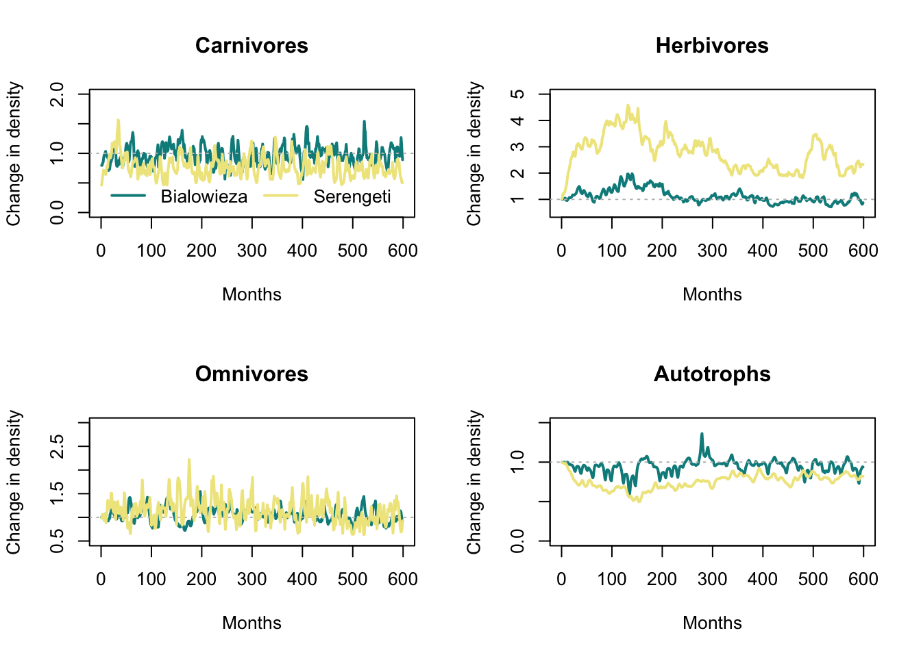

Let’s also compare the resulting food webs. Hoeks et al. (2020) found that large herbivores increased in biomass after large carnivore removal, especially in the Serengeti; the biomass of medium-sized endothermic carnivores (10-21kg) was increased; the biomass of large (>100 kg) endothermic omnivores decreased. Compare to our simulation results below.

# Plot foodweb plot
par(mfrow=c(1,1))
plot_foodweb(mres_control_B, max_flows = 5)

## loading inputs from: /Users/zurell/data/Lehre/UP_Lehre/CLEWS/EcosystemDynamics/edb-course/models/Mad_carnivores/madingley_outs_31_05_22_20_01_50/

title('Bialowieza - control scenario')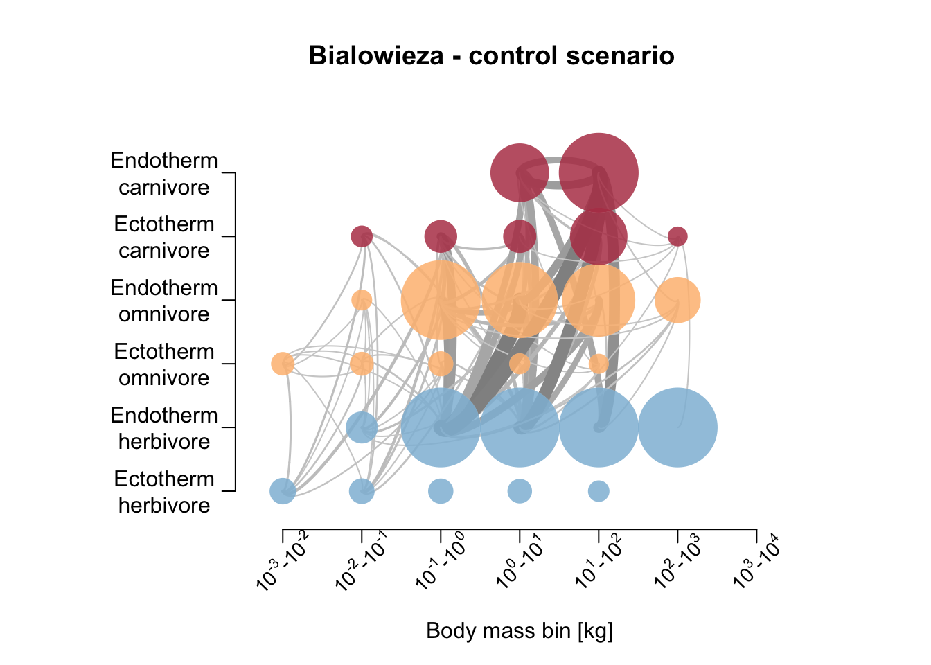

plot_foodweb(mres_removal_B, max_flows = 5)

## loading inputs from: /Users/zurell/data/Lehre/UP_Lehre/CLEWS/EcosystemDynamics/edb-course/models/Mad_carnivores/madingley_outs_31_05_22_20_10_35/

title('Bialowieza - removal scenario')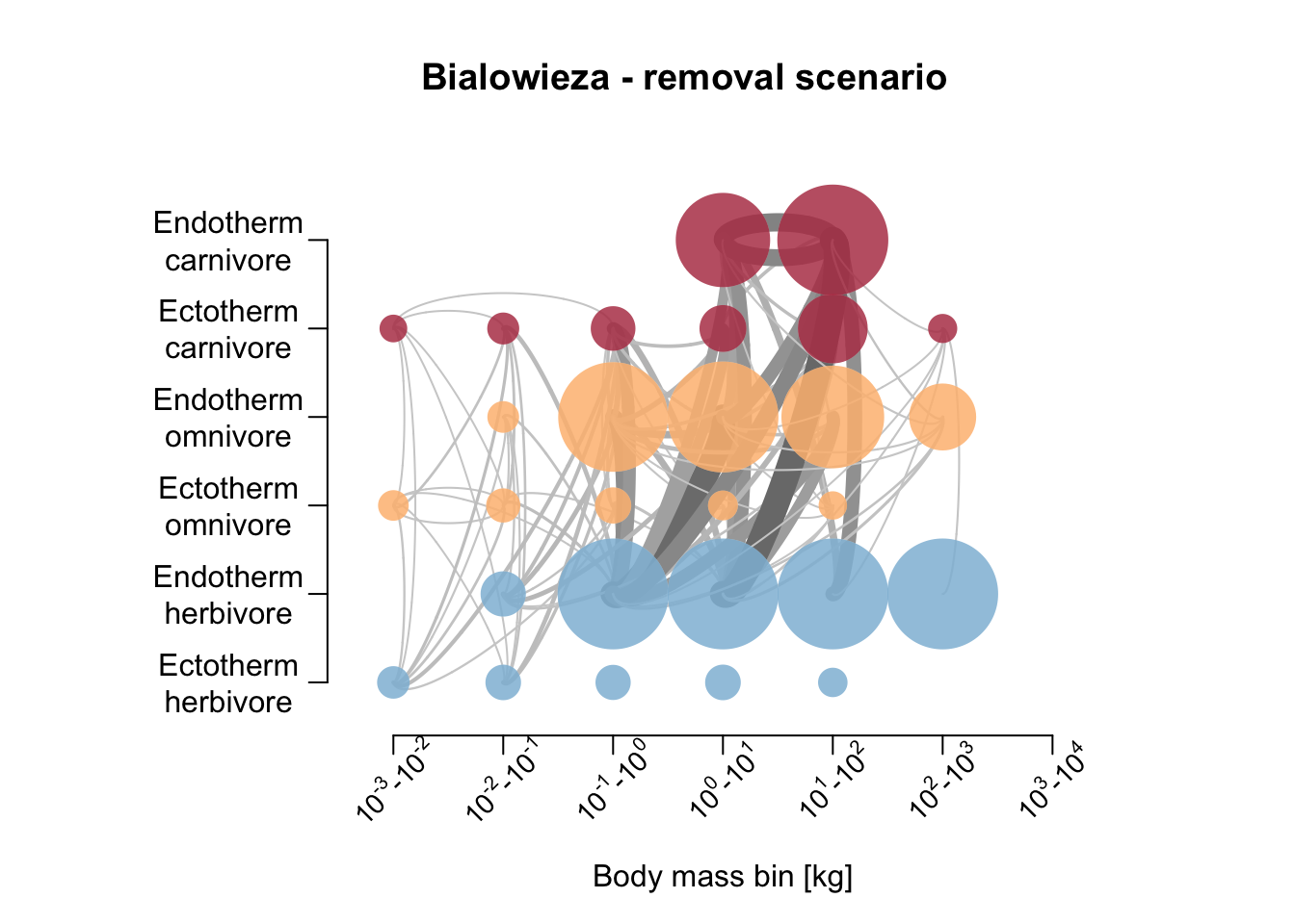

plot_foodweb(mres_control_S, max_flows = 5)

## loading inputs from: /Users/zurell/data/Lehre/UP_Lehre/CLEWS/EcosystemDynamics/edb-course/models/Mad_carnivores/madingley_outs_29_06_22_11_33_27/

title('Serengeti - control scenario')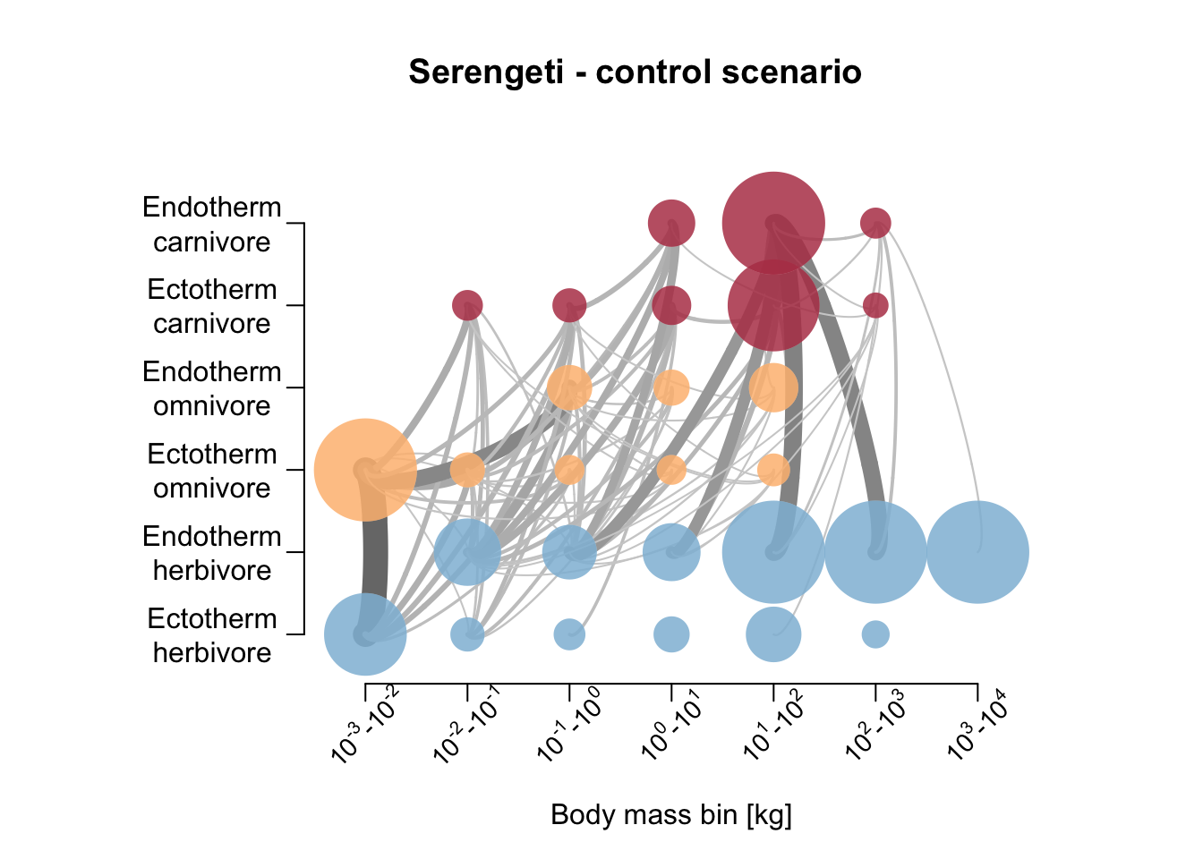

plot_foodweb(mres_removal_S, max_flows = 5)

## loading inputs from: /Users/zurell/data/Lehre/UP_Lehre/CLEWS/EcosystemDynamics/edb-course/models/Mad_carnivores/madingley_outs_31_05_22_20_13_49/

title('Serengeti - removal scenario')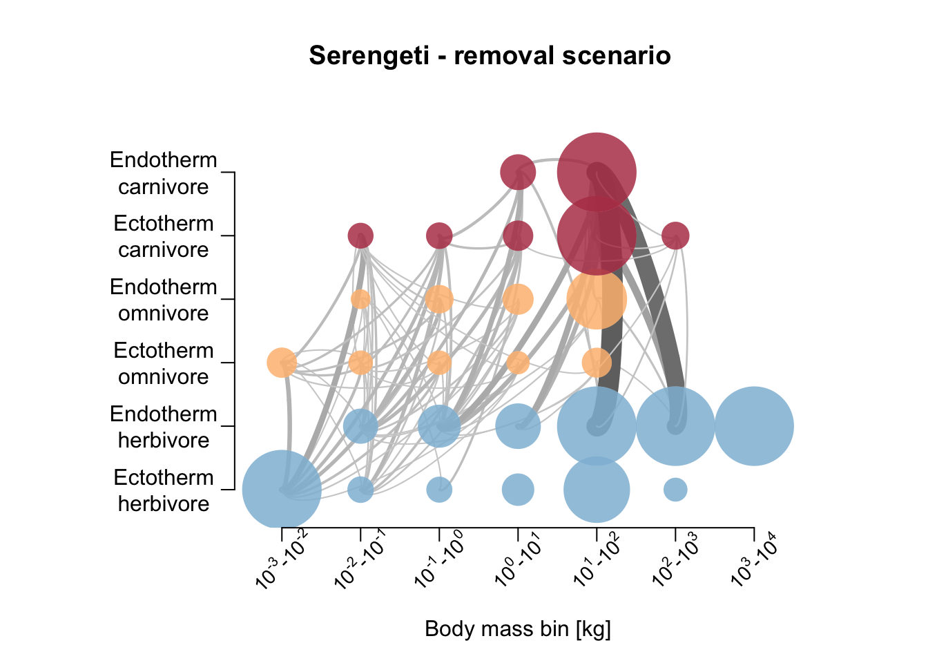

# Plot body mass densities
par(mfcol=c(3,2))
hist(subset(mres_control_B$cohorts, FunctionalGroupIndex==0)$AdultMass/1000, main='Bialowieza control - herbivores', xlab='Body mass [kg]')
hist(subset(mres_control_B$cohorts, FunctionalGroupIndex==1)$AdultMass/1000, main='Bialowieza control - carnivores', xlab='Body mass [kg]')
hist(subset(mres_control_B$cohorts, FunctionalGroupIndex==2)$AdultMass/1000, main='Bialowieza control - omnivores', xlab='Body mass [kg]')
hist(subset(mres_removal_B$cohorts, FunctionalGroupIndex==0)$AdultMass/1000, main='Bialowieza removal - herbivores', xlab='Body mass [kg]')
hist(subset(mres_removal_B$cohorts, FunctionalGroupIndex==1)$AdultMass/1000, main='Bialowieza removal - carnivores', xlab='Body mass [kg]')
hist(subset(mres_removal_B$cohorts, FunctionalGroupIndex==2)$AdultMass/1000, main='Bialowieza removal - omnivores', xlab='Body mass [kg]')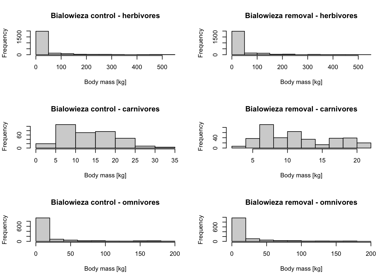

par(mfcol=c(3,2))
hist(subset(mres_control_S$cohorts, FunctionalGroupIndex==0)$AdultMass/1000, main='Serengeti control - herbivores', xlab='Body mass [kg]')
hist(subset(mres_control_S$cohorts, FunctionalGroupIndex==1)$AdultMass/1000, main='Serengeti control - carnivores', xlab='Body mass [kg]')
hist(subset(mres_control_S$cohorts, FunctionalGroupIndex==2)$AdultMass/1000, main='Serengeti control - omnivores', xlab='Body mass [kg]')
hist(subset(mres_removal_S$cohorts, FunctionalGroupIndex==0)$AdultMass/1000, main='Serengeti removal - herbivores', xlab='Body mass [kg]')
hist(subset(mres_removal_S$cohorts, FunctionalGroupIndex==1)$AdultMass/1000, main='Serengeti removal - carnivores', xlab='Body mass [kg]')
hist(subset(mres_removal_S$cohorts, FunctionalGroupIndex==2)$AdultMass/1000, main='Serengeti removal - omnivores', xlab='Body mass [kg]')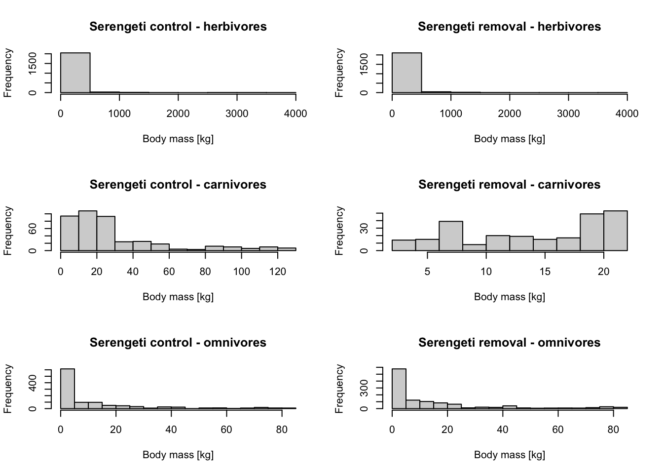

Task: extend analyses

Now, it’s your turn. Test other locations from Hoeks et al. (2020). Or implement several replicates and compare results.

References

Dirzo, Rodolfo, Hillary S. Young, Mauro Galetti, Gerardo Ceballos, Nick J. B. Isaac, and Ben Collen. 2014. “Defaunation in the Anthropocene.” Science 345 (6195): 401–6. https://doi.org/10.1126/science.1251817.

Hoeks, Selwyn, Mark A. J. Huijbregts, Michela Busana, Michael B. J. Harfoot, Jens-Christian Svenning, and Luca Santini. 2020. “Mechanistic Insights into the Role of Large Carnivores for Ecosystem Structure and Functioning.” Ecography 43 (12): 1752–63. https://doi.org/10.1111/ecog.05191.

Svenning, Jens-Christian, Pil B. M. Pedersen, C. Josh Donlan, Rasmus Ejrnæs, Søren Faurby, Mauro Galetti, Dennis M. Hansen, et al. 2016. “Science for a Wilder Anthropocene: Synthesis and Future Directions for Trophic Rewilding Research.” Proceedings of the National Academy of Sciences 113 (4): 898–906. https://doi.org/10.1073/pnas.1502556112.

MadingleyR: Role of large carnivores