Pseudo-absence and background data
RStudio project
Open the RStudio project that we created in the first session. I recommend to use this RStudio project for the entire course and within the RStudio project create separate R scripts for each session.
- Create a new empty R script by going to the tab “File”, select “New File” and then “R script”
- In the new R script, type
# Session b5: Pseudo-absence and background dataand save the file in your folder “scripts” within your project folder, e.g. as “b5_PseudoAbsences.R”
1 Introduction
In the previous sessions, we have worked with very convenient presence/absence data to train our species distribution models (SDMs). However, as you have seen when downloading your own GBIF data, we often have only presence records available. Absence data are also inherently difficult to get because it requires a very high sampling effort to classify a species as absent from a location. For plants, we would need complete inventories of a larger region, e.g. several 100 m plots placed within larger 1 km sample squares. For birds, we would need several visits to a specific region within the breeding season. In both cases, we could still miss some species, meaning that we do not record the species although present (resulting in a false negative).
But what should we do if absence data are not available? Most SDM algorithms (except the profile methods, see session 6) need some kind of absence or background data to contrast the presence data to. There are different approaches for creating background data or pseudo-absence data (Barbet-Massin et al. 2012; Kramer-Schadt et al. 2013; Phillips et al. 2009), although there is still room for further developments in this field and more clear-cut recommendations for users would be certainly useful. Nevertheless, I hope this tutorial will provide some examples of how to deal with presence-only data. For advice on how many background/pseudo-absence points you need, please read (Barbet-Massin et al. 2012).
In this session, we look at two major ways of creating background/pseudo-absence data:
- random selection of points within study area (including or excluding the presence locations) (Barbet-Massin et al. 2012)
- random selection of points outside of study area (Barbet-Massin et al. 2012)
We will not cover approaches for dealing with sampling bias:
- accounting for spatial sampling bias using target-group selection (Phillips et al. 2009)
- accounting for spatial sampling bias using inverse distance weighting (Kramer-Schadt et al. 2013)
At the end of the practical, I provide an exemplary workflow for selecting pseudo-absence data for our own GBIF data (using the Alpine shrew), for spatially thinning these data and for merging with environmental data.
2 Species presence data
I created a virtual species data set with presence points for a dummy species called Populus imagines and sister species Populus spp. The spatial resolution of the data is 5 minutes. You can download the data here or from the moodle page.
Load and plot the data:
library(terra)

# Our study region and species data
region <- terra::rast('data/Prac5_Europe5min.grd') # mask of study region
sp <- read.table('data/Prac5_presences.txt', header=T) # species presences

# Plot the map and data
plot(region,col='grey',legend=F)
points(sp[sp$sp=='Populus_imagines',1:2],pch='+',col='red')
points(sp[sp$sp=='Populus_spp',1:2],pch='+',cex=0.3,col='grey20')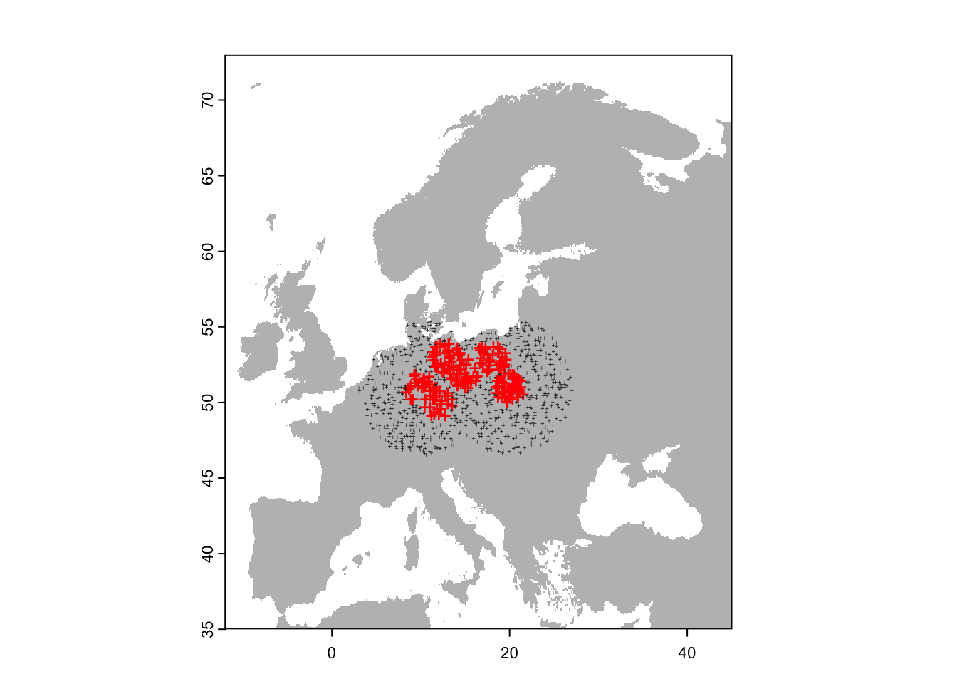
3 Background/Pseudo-absence data selection
We use a lot of methods from the predicts and
terra tutorials, which are worth looking into (see link
here).
3.1 Random selection of points within study area but excluding the presence location
The terra package has a function
spatSample() to sample random points (background data). In
the following examples, we aim to sample 500 pseudo-absence / background
data points.
# Randomly select background points from study region
# The argument na.rm=T ensures that we only sample points within the masked regions (not in the ocean)
# The argument as.points=T indicates that a SpatVector of coordinates should be returned
bg_rand <- terra::spatSample(region, 500, "random", na.rm=T, as.points=TRUE)

# Plot the map and data
plot(region,col='grey',legend=F)
points(sp[sp$sp=='Populus_imagines',1:2],pch='+',col='red')
points(bg_rand,pch=19,cex=0.3)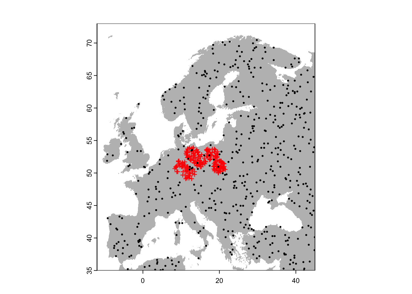
By default the function spatSample() will sample from
the entire study area independent of the presence points - corresponding
to the idea of background data. In order not to sample pseudo-absence at
presence locations, we have to tweak our regional mask and assign
NA to the presence location
# Make a new regional mask that contains NAs in presence locations:
sp_cells <- terra::extract(region, sp[sp$sp=='Populus_imagines',1:2], cells=T)$cell
region_exclp <- region
values(region_exclp)[sp_cells] <- NA

# Randomly select background data but excluding presence locations
bg_rand_exclp <- terra::spatSample(region_exclp, 500, "random", na.rm=T, as.points=TRUE)

# Plot the map and data
plot(region,col='grey',legend=F)
points(sp[sp$sp=='Populus_imagines',1:2],pch='+',col='red')
points(bg_rand_exclp,pch=19,cex=0.3)
Also, we can define an extent from where random points should be drawn.
# Define extent object:
e <- ext(8,24,46,57)

# Randomly select background data within a restricted extent and excluding presence locations:
bg_rand_exclp_e <- terra::spatSample(region_exclp, 500, "random", na.rm=T, as.points=TRUE, ext=e)

# Plot the map and data
plot(region,col='grey',legend=F)
points(sp[sp$sp=='Populus_imagines',1:2],pch='+',col='red')
points(bg_rand_exclp_e,pch=19,cex=0.3)
lines(e, col='red')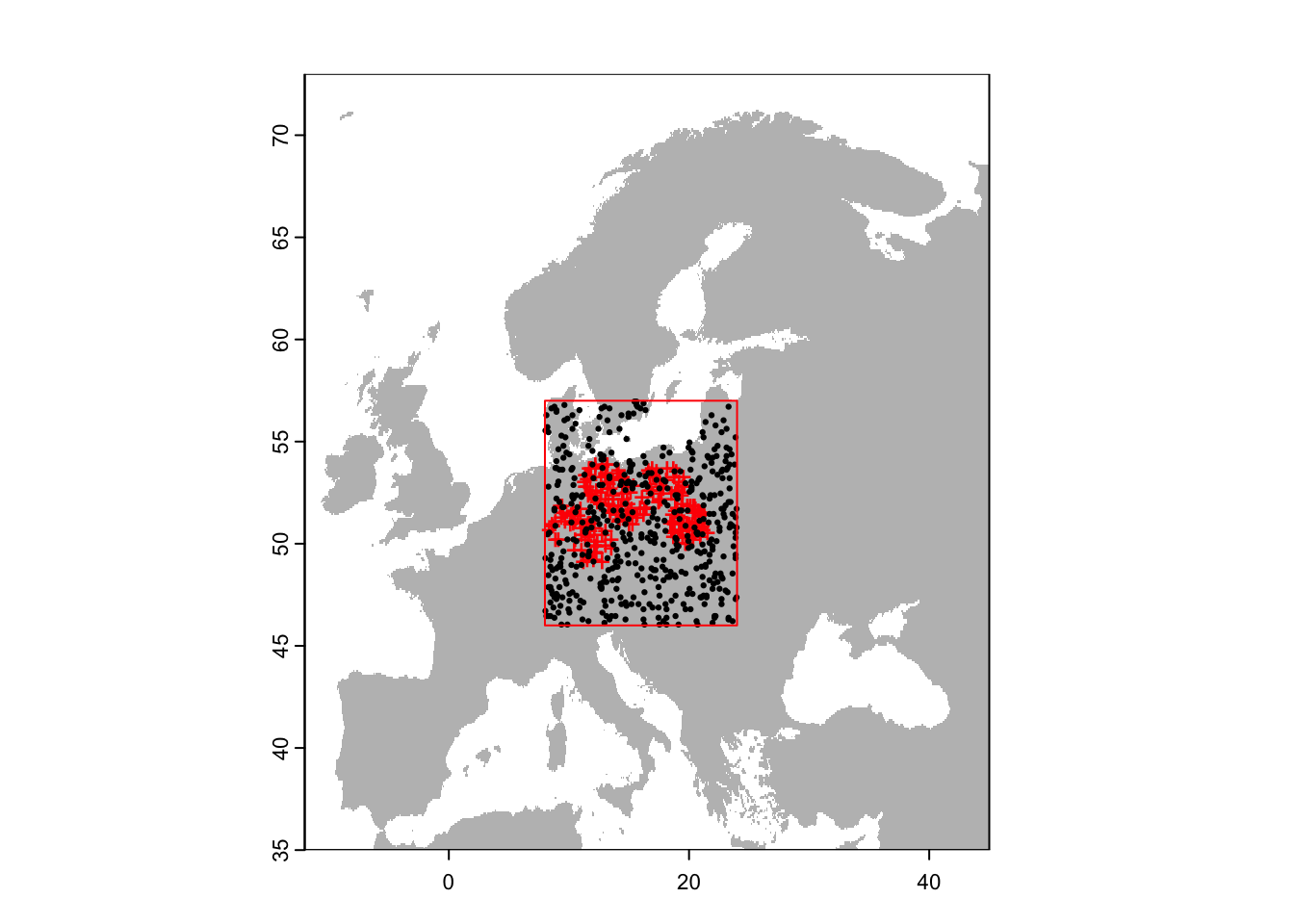
Last, we could also restrict the random samples to within a certain
buffer distance. For this, we first create a SpatVector,
then place a buffer around these and sample from within the buffer. The
buffer can be interpreted as the area that was accessible to the species
in the long-term past. Thus, the buffer helps accounting for
biogeographic history by constraining background/pseudo-absence points
to those geographic area that could have been reached by the species
given the movement capacity but excludes other areas. Of course,
restricting the absences to a certain geographic rectangle can achieve a
similar tasks but might be less accurate for complex geographies and
large areas. For example, is Iceland accessible to European species or
not?
# Create SpatVector object of known occurrences:
pop_imag <- terra::vect( as.matrix( sp[sp$sp=='Populus_imagines',1:2]) , crs=crs(region))

# Then, place a buffer of 200 km radius around our presence points
v_buf <- terra::buffer(pop_imag, width=200000)

# Set all raster cells outside the buffer to NA
region_buf <- terra::mask(region, v_buf)

# Randomly select background data within the buffer
bg_rand_buf <- terra::spatSample(region_buf, 500, "random", na.rm=T, as.points=TRUE)

# Plot the map and data
plot(region,col='grey',legend=F)
plot(region_buf, legend=F, add=T)
points(sp[sp$sp=='Populus_imagines',1:2],pch='+',col='red')
points(bg_rand_buf,pch=19,cex=0.3)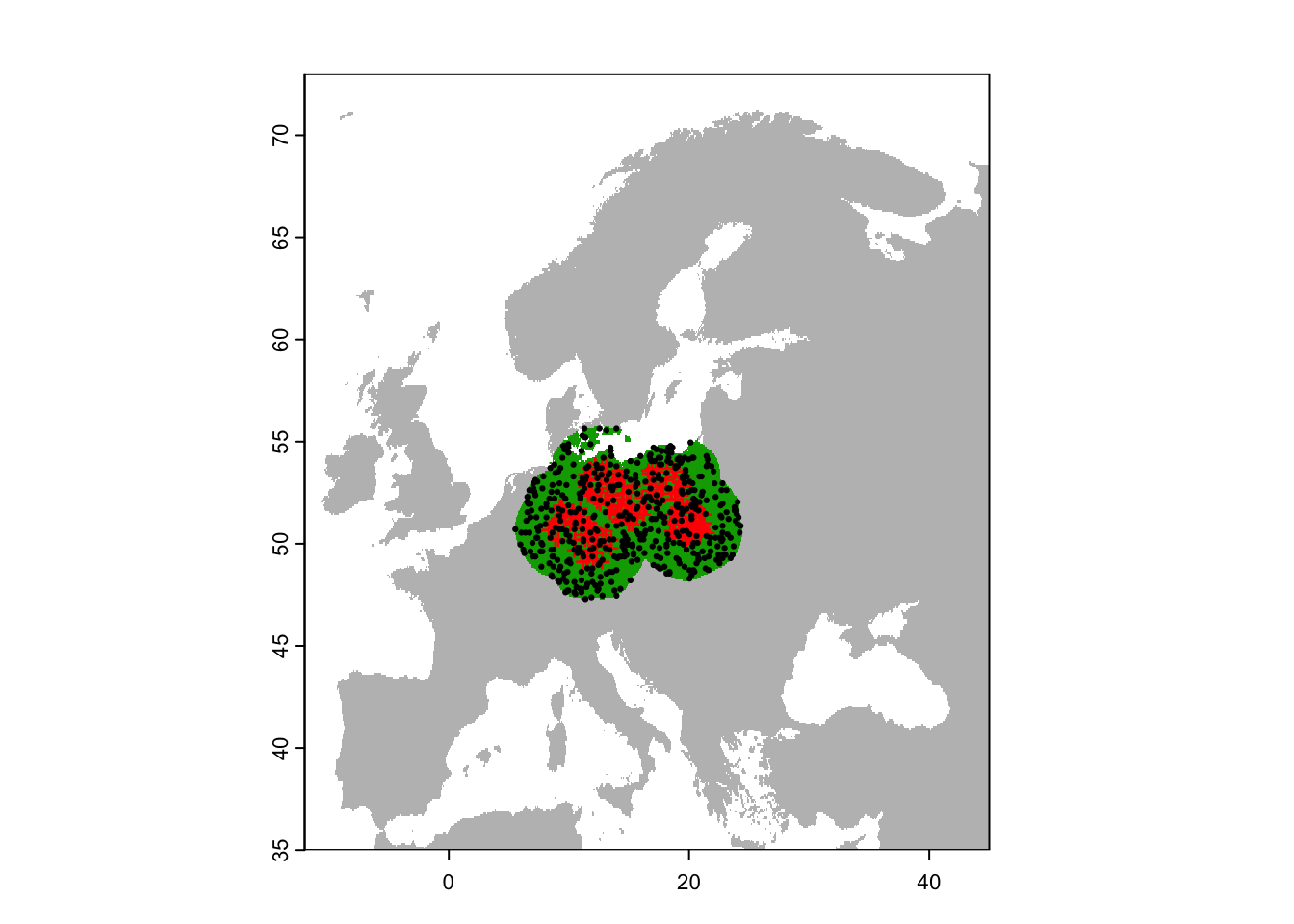
3.2 Random selection of points outside of study area
Barbet-Massin et al. (2012) also suggested a method to sample pseudo-absences only beyond a minimum distance from the presence points. This is more of a macroecological approach, suitable for characterising the climatic limits of species. We can also use the buffering approach from above to achieve this.
# Place a buffer of 200 km radius around our presence points
v_buf <- terra::buffer(pop_imag, width=200000)

# Set all raster cells inside the buffer to NA using the argument inverse=T
region_outbuf <- terra::mask(region, v_buf, inverse=T)
region_buf <- terra::mask(region, v_buf)  # we use this only for illustrative purpose below

# Randomly select background data outside the buffer
bg_rand_outbuf <- terra::spatSample(region_outbuf, 500, "random", na.rm=T, as.points=TRUE)

# Plot the map and data
plot(region,col='grey',legend=F)
plot(region_buf,legend=F, add=T)
points(sp[sp$sp=='Populus_imagines',1:2],pch='+',col='red')
points(bg_rand_outbuf,pch=19,cex=0.3)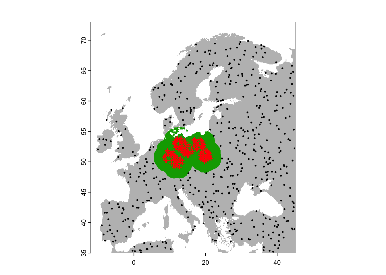
4 Workflow for joining presence and background/pseudo-absence data
In session b2, we have already learned how to join species data and environmental data (at 10 min resolution) using the Alpine shrew as example species. Here, we will revisit this example, sample random background data and join these with environmental data to come up with a dataset containing presences and background data as well as the climatic predictors.
# Load the species presence data (here, the data set from session 1):
load('data/gbif_shrew_cleaned.RData')

head(gbif_shrew_cleaned[,1:4])
## key scientificName decimalLatitude decimalLongitude
## 1 4880822152 Sorex alpinus Schinz, 1837 47.77657 13.214792
## 2 4926239461 Sorex alpinus Schinz, 1837 46.50952 8.844546
## 3 4851859068 Sorex alpinus Schinz, 1837 46.39773 12.171057
## 4 4901479303 Sorex alpinus Schinz, 1837 47.44663 10.976726
## 5 4901510667 Sorex alpinus Schinz, 1837 47.44961 10.876853
## 6 4875417397 Sorex alpinus Schinz, 1837 46.57841 7.778424# Plot the species presences
library(maps)
maps::map('world',xlim=c(-12,45), ylim=c(35,73))
points(gbif_shrew_cleaned$decimalLongitude, gbif_shrew_cleaned$decimalLatitude, col='red', pch=19)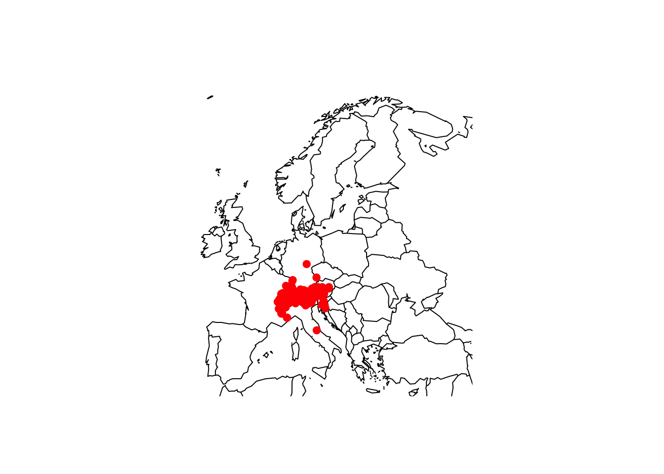
You have already downloaded the climate data at 10-min spatial resolution in session b2 and can simply read it back in. We crop it to European extent.
library(geodata)

# Download global bioclimatic data from worldclim (you may have to set argument 'download=T' for first download, if 'download=F' it will attempt to read from file):
clim <- geodata::worldclim_global(var = 'bio', res = 10, download = F, path = 'data')

# Crop to Europe
clim <- terra::crop(clim, c(-12,45,35,73))
What is important to consider is that you kind of arbitrarily choose a scale of analysis by choosing climate data (or other environmental data) at a certain spatial resolution. Here, we choose a spatial resolution of 10 minutes while the species data may actually be at a finer resolution. So, we first make sure that our species data are fit to the spatial resolution, meaning we remove any duplicates within 10 minute cells. We do this by joining the species data with the environmental data (basically, repeating what we had already done at the end of session b2). Then, we can remove the duplicate cells.
# Extract raster cellnumbers for the species data
gbif_shrew_dat <- data.frame(gbif_shrew_cleaned[,1:4], cell=terra::cellFromXY(clim, as.matrix(gbif_shrew_cleaned[,c('decimalLongitude','decimalLatitude')])))

# Remember to remove any rows with duplicate cellnumbers if necessary:
sum(duplicated(gbif_shrew_dat$cell))
## [1] 209# Only retain non-duplicated cells
gbif_shrew_dat <- gbif_shrew_dat[!duplicated(gbif_shrew_dat$cell),]
# From now on, we just need the coordinates:
gbif_shrew_coords <- gbif_shrew_dat[,c('decimalLongitude','decimalLatitude')]We place a buffer of 200 km around the shrew records and sample background points randomly from within the buffer but excluding presence locations (remember that also other pseudo-absence/background data strategies are possible). We sample three times as many background data points as we have presences. Strictly, we should use ten times as many background points (Barbet-Massin et al. 2012), but we use a multiplier of three here for simplicity.
# Make SpatVector:
presences <- terra::vect( as.matrix(gbif_shrew_coords), crs=crs(clim))

# Then, place a buffer of 200 km radius around our presence points
v_buf <- terra::buffer(presences, width=200000)

# Create a background mask with target resolution and extent from climate layers
# Set all raster cells outside the buffer to NA.
bg <- clim[[1]]
values(bg)[!is.na(values(bg))] <- 1
region_buf <- terra::mask(bg, v_buf)
plot(bg, col='grey90', legend=F)
plot(region_buf, add=T, col='grey60', legend=F)

# Exclude presence locations:
sp_cells <- terra::extract(region_buf, presences, cells=T)$cell
region_buf_exclp <- region_buf
values(region_buf_exclp)[sp_cells] <- NA

# Randomly select background data within the buffer, excluding presence locations. We sample 3 times as many background data as we have presences. To ensure that we find enough samples, we use the argument exhaustive=T
bg_rand_buf <- terra::spatSample(region_buf_exclp, length(presences)*3, "random", na.rm=T, as.points=TRUE, exhaustive=T)

points(bg_rand_buf, pch=19, cex=0.2)
points(presences, pch=19, cex=0.5, col='red')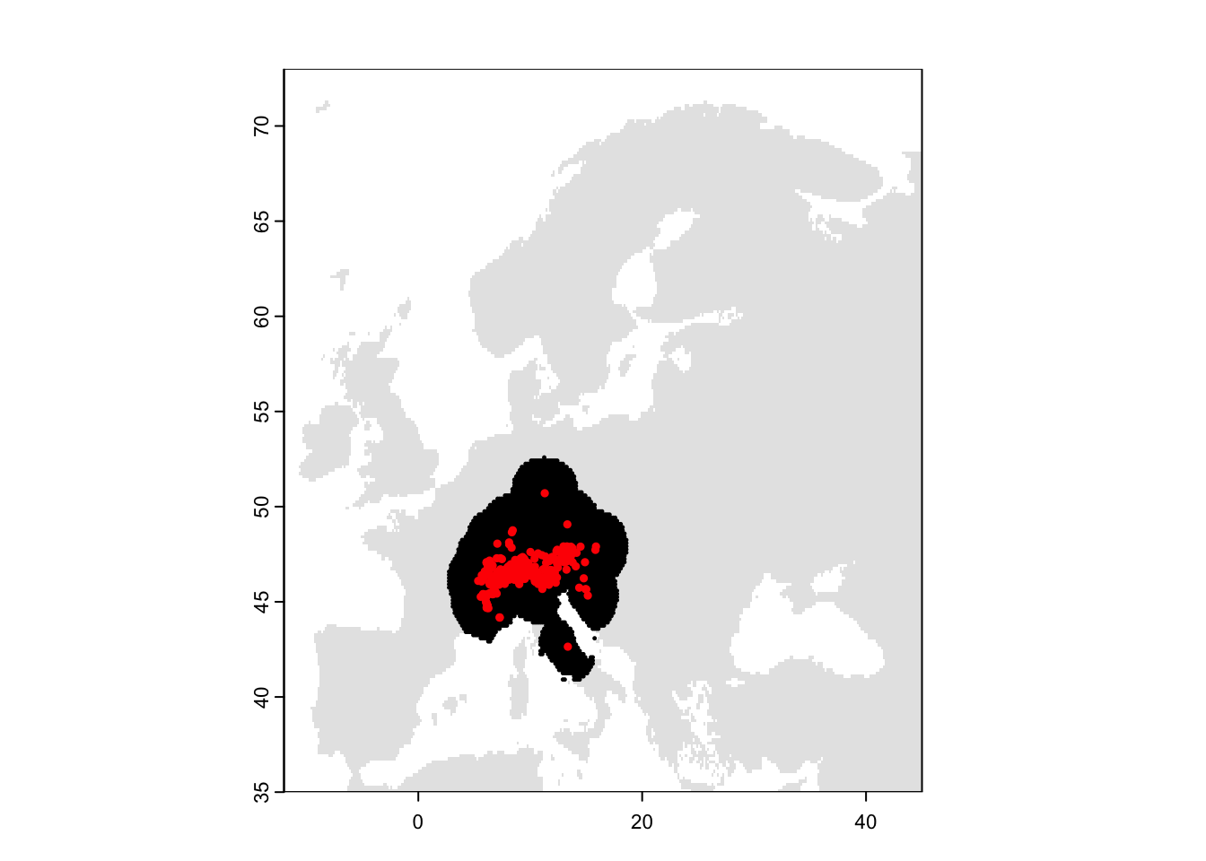
Next, we need to join the presences and background data, and extract the environmental data.
# First, we prepare the presences data to contain a column indicating 1 for presence.
sp_env <- data.frame(gbif_shrew_coords, occ=1)

# Second, we make sure the background data have the same columns, and indicate 0 for absence.
bg_rand_buf_df <- data.frame(terra::geom(bg_rand_buf)[,c('x','y')])
summary(bg_rand_buf_df)
## x y
## Min. : 2.75 Min. :40.92
## 1st Qu.: 9.75 1st Qu.:44.92
## Median :14.25 Median :47.42
## Mean :13.70 Mean :47.17
## 3rd Qu.:17.92 3rd Qu.:49.42
## Max. :23.58 Max. :52.58names(bg_rand_buf_df) <- c('decimalLongitude','decimalLatitude')
bg_rand_buf_df$occ <- 0
summary(bg_rand_buf_df)## decimalLongitude decimalLatitude occ
## Min. : 2.75 Min. :40.92 Min. :0
## 1st Qu.: 9.75 1st Qu.:44.92 1st Qu.:0
## Median :14.25 Median :47.42 Median :0
## Mean :13.70 Mean :47.17 Mean :0
## 3rd Qu.:17.92 3rd Qu.:49.42 3rd Qu.:0
## Max. :23.58 Max. :52.58 Max. :0# Third, we bind these two data sets
sp_env <- rbind(sp_env, bg_rand_buf_df)
summary(sp_env)## decimalLongitude decimalLatitude occ
## Min. : 2.750 Min. :40.92 Min. :0.00
## 1st Qu.: 8.917 1st Qu.:45.42 1st Qu.:0.00
## Median :12.917 Median :47.01 Median :0.00
## Mean :12.953 Mean :47.10 Mean :0.25
## 3rd Qu.:17.083 3rd Qu.:48.92 3rd Qu.:0.25
## Max. :23.583 Max. :52.58 Max. :1.00# Last, we join this combined data set with the climate data.
sp_env <- cbind(sp_env, terra::extract(x = clim, y = sp_env[,c('decimalLongitude','decimalLatitude')], cells=T) )
summary(sp_env)## decimalLongitude decimalLatitude occ ID
## Min. : 2.750 Min. :40.92 Min. :0.00 Min. : 1.0
## 1st Qu.: 8.917 1st Qu.:45.42 1st Qu.:0.00 1st Qu.: 276.8
## Median :12.917 Median :47.01 Median :0.00 Median : 552.5
## Mean :12.953 Mean :47.10 Mean :0.25 Mean : 552.5
## 3rd Qu.:17.083 3rd Qu.:48.92 3rd Qu.:0.25 3rd Qu.: 828.2
## Max. :23.583 Max. :52.58 Max. :1.00 Max. :1104.0
## wc2.1_10m_bio_1 wc2.1_10m_bio_2 wc2.1_10m_bio_3 wc2.1_10m_bio_4
## Min. :-2.835 Min. : 5.325 Min. :24.74 Min. :532.6
## 1st Qu.: 6.580 1st Qu.: 8.077 1st Qu.:30.83 1st Qu.:628.4
## Median : 8.289 Median : 8.592 Median :32.28 Median :679.0
## Mean : 8.109 Mean : 8.632 Mean :32.24 Mean :682.3
## 3rd Qu.:10.029 3rd Qu.: 9.261 3rd Qu.:33.66 3rd Qu.:727.6
## Max. :16.663 Max. :11.592 Max. :39.49 Max. :871.5
## wc2.1_10m_bio_5 wc2.1_10m_bio_6 wc2.1_10m_bio_7 wc2.1_10m_bio_8
## Min. : 8.959 Min. :-13.749 Min. :19.90 Min. :-6.303
## 1st Qu.:20.813 1st Qu.: -5.783 1st Qu.:25.06 1st Qu.: 9.647
## Median :23.213 Median : -4.194 Median :26.79 Median :14.441
## Mean :22.679 Mean : -4.079 Mean :26.76 Mean :12.626
## 3rd Qu.:25.253 3rd Qu.: -2.528 3rd Qu.:28.46 3rd Qu.:16.989
## Max. :31.481 Max. : 8.000 Max. :32.74 Max. :21.641
## wc2.1_10m_bio_9 wc2.1_10m_bio_10 wc2.1_10m_bio_11 wc2.1_10m_bio_12
## Min. :-9.4345 Min. : 4.412 Min. :-9.4345 Min. : 309.0
## 1st Qu.:-0.4836 1st Qu.:14.809 1st Qu.:-1.8550 1st Qu.: 675.0
## Median : 1.7168 Median :17.044 Median :-0.3963 Median : 883.5
## Mean : 3.7692 Mean :16.541 Mean :-0.1374 Mean : 936.8
## 3rd Qu.: 5.2482 3rd Qu.:18.669 3rd Qu.: 1.5351 3rd Qu.:1172.0
## Max. :25.0329 Max. :25.033 Max. :10.8833 Max. :2127.0
## wc2.1_10m_bio_13 wc2.1_10m_bio_14 wc2.1_10m_bio_15 wc2.1_10m_bio_16
## Min. : 39.0 Min. : 8.00 Min. : 4.41 Min. :107.0
## 1st Qu.: 85.0 1st Qu.: 31.75 1st Qu.:18.79 1st Qu.:233.0
## Median :104.0 Median : 49.00 Median :26.13 Median :286.0
## Mean :112.3 Mean : 50.55 Mean :26.36 Mean :310.6
## 3rd Qu.:134.0 3rd Qu.: 65.00 3rd Qu.:33.67 3rd Qu.:373.0
## Max. :239.0 Max. :114.00 Max. :60.26 Max. :663.0
## wc2.1_10m_bio_17 wc2.1_10m_bio_18 wc2.1_10m_bio_19 cell
## Min. : 36.0 Min. : 45.0 Min. : 36.0 Min. :41896
## 1st Qu.:108.8 1st Qu.:205.0 1st Qu.:122.8 1st Qu.:49436
## Median :165.0 Median :245.0 Median :187.0 Median :53208
## Mean :169.9 Mean :273.2 Mean :195.5 Mean :53133
## 3rd Qu.:217.0 3rd Qu.:325.5 3rd Qu.:249.0 3rd Qu.:56536
## Max. :404.0 Max. :573.0 Max. :526.0 Max. :658154.1 Spatial thinning
When we prepare our distribution data for species distribution modelling, we also need to think about spatial autocorrelation. Using adjacent cells in model building can lead to problems with spatial autocorrelation. As a rule of thumb, data points should be at least 2-3 cells apart.
One way to avoid this is spatially thinning the records, for example
using the package spThin (Aiello-Lammens et al. 2015). Load the package
and look up the help page ?thin.
library(spThin)

# The spThin package requires longitude/latitude coordinates, which we already have.
# Look up the help page and try to understand the function:
?thin

# thin() expects that the data.frame contains a column with the species name
sp_env$sp <- 'Sorex_alpinus'

# Remove adjacent cells of presence/background data:
xy <- thin(sp_env, lat.col='decimalLatitude',long.col='decimalLongitude',spec.col='sp', thin.par=30,reps=1, write.files=F,locs.thinned.list.return=T)
## **********************************************
## Beginning Spatial Thinning.
## Script Started at: Tue Oct 22 20:30:02 2024
## lat.long.thin.count
## 539
## 1
## [1] "Maximum number of records after thinning: 539"
## [1] "Number of data.frames with max records: 1"
## [1] "No files written for this run."# Keep the coordinates with the most presence records
xy_keep <- xy[[1]]
# Thin the dataset - here, we first extract the cell numbers for the thinned coordinates and then use these to subset our data frame.
cells_thinned <- terra::cellFromXY(clim, xy_keep)
sp_thinned <- sp_env[sp_env$cell %in% cells_thinned,]
# Plot the map and data
plot(bg, col='grey90', legend=F)
points(sp_thinned[,1:2],pch=19,col=c('black','red')[as.factor(sp_thinned$occ)], cex=0.3)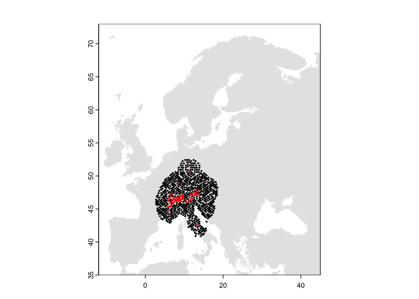
Finally, don’t forget to save your data, for example by writing the final data frame to file or by saving the R object(s).
save(sp_thinned,file='data/gbif_shrew_PresAbs_thinned.RData')Alternative: The thin() function can
take quite long and needs a lot of memory space. Alternatively, we can
use the terra package to thin the data to a checkerboard
pattern, i.e. remove every second cell.
# Create checkerboard SpatRaster
r_chess <- mask(init(region_buf,'chess'), region_buf)
values(r_chess)[values(r_chess)<1] <- NA
names(r_chess) <- 'chess'

# Thinning to the checkerboard pattern
sp_thinned2 <- merge(as.data.frame(r_chess,cell=T),sp_env,by='cell')

# Plot the map and data
plot(bg, col='grey90', legend=F)
points(sp_thinned2[,c('decimalLongitude','decimalLatitude')],pch=19,col=c('black','red')[as.factor(sp_thinned2$occ)], cex=0.3)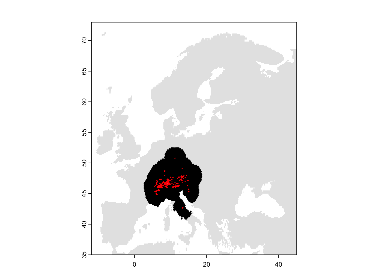
These different thinning methods of coarse result in very different number of presences and absences retained.
# spThin function
table(sp_thinned$occ)
##
## 0 1
## 457 82# checkerboard at original spatial resolution
table(sp_thinned2$occ)##
## 0 1
## 432 1355 Homework prep
As homework, solve the exercises in the blue box below.
Exercise:
In practical b1, you have downloaded your own GBIF data. Carry out the pseudo-absence data selection for this species, and run a GLM analysis.
- Decide on a pseudo-absence/background data strategy for your species (in the simplest case, just follow the strategy used in the example workflow in section 4). Prepare your dataset with presences, pseudo-absences and the corresponding climate data at those locations (following the workflow in section 4)
- Use the data and build a GLM. Remember the different steps of checking for multicollinearity, building the full model and simplifying it (cf. practical b3).
- Assess the predictive performance of that model (cf. practical b4).
- Make predictions to current climate. Decide whether you want to make predictions to the entire globe or to a more restricted geographic area (e.g. the continent where your species occurs)?